Learning – how to measure plant functional traits – the hard way (a story in 4, or more, parts)
TraitTrain is a group of plant ecologists from the Universities of Bergen in Norway and Arizona (USA). We want to strengthen research and educational collaborations over climate change and ecosystem ecology. We are organizing courses for students on how to measure plant functional traits and at the same time offer the students a relevant research experience, i.e. by being part of a real research project and collecting real data. Being part of a projects is more motivating for students than collecting “dummy data”. This is a challenging goal and does not always work out. Here, I want to explain how we organize these courses and what we learned from our mistakes. In a couple of next blog posts, I want to discuss how to ensure data quality, technical problems and solutions, next steps and unresolved problems.
On our team, we have an extremely successful person getting research grants (basically our boss), and she is also obsessed with education and collecting all sorts of data. She secured the money to organize the trait courses. Also, we have many colleagues who were willing to travel to cool places (China, Peru, Svalbard) and teach functional trait and climate change ecology. Finally, we have hospitable Chinese, Peruvian, Icelandic and Norwegian collaborators with field sites at the edge of the Tibetan Plateau (Sichuan, China), in the Andes (Peru) and Svalbard (Longyearbyen, “Norway”) willing to let a hoard of students lose on their field sites and experiments. Not sure, if I would…
What is the big deal with organizing a course with a couple of students? There is nothing special about that, and hundreds of people have done this before. The special thing with our courses was, that we did not only want to teach about traits and climate change ecology; we also wanted to collect a publishable data set. And this is where it gets tricky. The good thing about all the students is that a huge amount of data can be collected in a short time. The downside, it can go horribly wrong and instructions need to be given very explicitly to collect the data in a standardized way. The problems can be passed along from one student to the next and errors accumulate.
The basic principle of measuring leaf traits is to go to the field, collect plants, bring them back to the lab where traits are measured (see video below): plant height, wet mass, leaf area, thickness. Then the leaves are dried and weighed again for dry mass. From the dry leaves, chemical traits for example carbon and nitrogen content can be measured. To get a decent data sets, you need trait measurements from different species, leaves and locations, and you will end up measuring hundreds of leaves. A tedious task! Our first strategy was the trait wheel, which has turned out to be very useful. The trait wheel is organizing the different trait measurements in separate stations and each leaf has to go through each station in a fixed order. And each station is manned by several students.
We followed the trait handbook by Pérez-Harguindeguy et al. (2013) and I am not repeating the basics of plant collections and trait measurements. Rather, I will highlight useful tips that we learnt from our mistakes.
The first step (not yet a station), is to collect the plants or leaves in the field. Where and how to collect leaves is important, but I will not go into detail here. This step depends on your research question and there are some useful guidelines on sampling strategies in the trait handbook. It is useful to measure plant height already in the field (unlike in the video!). Measuring plant height in the lab works well for “stiff” plants. But for plants that bend easily (e.g. grasses) it is hard to get the plant height right after the plant has been picked from the ground. We also found it useful to use a separate plastic bag for each plant. Yes, we used a lot of bags (we cleaned and reused the bags), but all information (date, site, species, height, collector, etc.) can be written directly on each bag and fewer plants get lost and information lost.
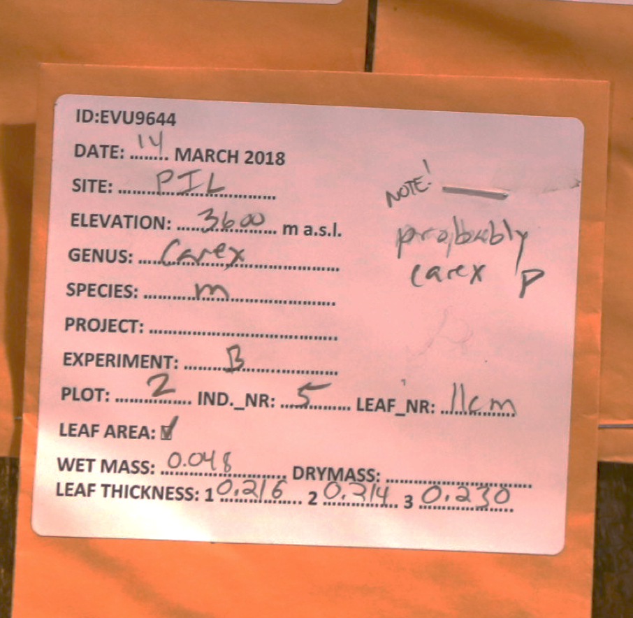
When a leaf arrives in the lab, it goes to station nr. 1 the preparation and labelling. Here, the plants are identified (if this has not already happened in the field), the leaves selected, put into an envelope and labelled. This is a crucial step and people with species identification skills are needed. Leaves that are labelled wrong or go in the wrong bag are difficult to fix later. Another point is to make sure, that each envelope is labelled with the necessary information. We learnt that even if you have to remember to note down the same 5 things, it is hard, and students (and professors) forget to write crucial information on the envelopes. To help the students to remember all information, we preprinted labels with blanks and boxes (see Photo). We used sticky labels that could be easily glued to each envelope. At each station, the data is entered or boxes are ticked. This reduced a large amount of errors.
Envelope with sticky label.
The preparation and labelling station is also when you decide how much plant material goes into one envelope. Usually one leaf is enough, but if the leaves are very small you might want to go for a bulk sample (several leaves from one individual). The amount of plant material is important for the chemical analysis where a certain amount of plant material is needed. Plan this step ahead and make sure you know how much plant material you need (dry weight!).
The next station is nr. 2 wet mass. This is not a particular difficult task. The important thing here is to have a balance that measures your leaves with sufficient accuracy. This is again important for small leaves, for example in arctic and alpine habitats.
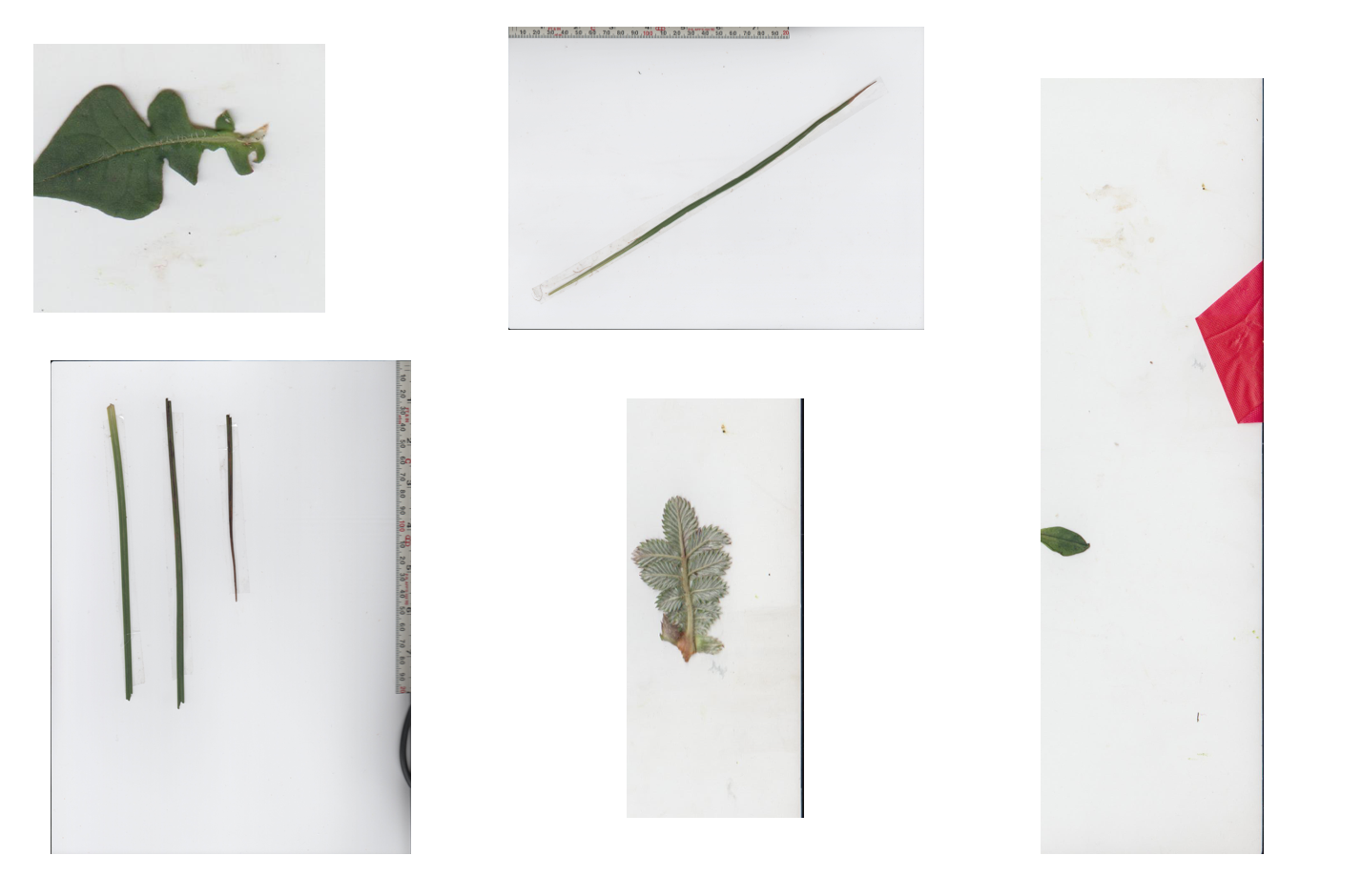
Station nr. 3 is scanning leaf area. A leaf is scanned using a normal scanner, and the area calculate using a software like ImageJ. It is important to scan the leaves upside down, scan the whole leaf (large leaves can be cut), keep leaves flat and not rolled (tape can be used to keep leaves flat) and not scan other things (e.g. cables, tissues; see photo). Keep the scanner clean at all times, because large dust and dirt particles will be counted as part of the leaf. And finally, have a ruler (to measure size) on each scan as reference object. There will be a separate blog post on the scanning process.
Different problems with leaf scans.
Station nr. 4 is measuring leaf thickness. A digital caliper should be used and this step will take a lot of time. It is good to have 3-4 people working on this at all times.
Next the leaves go into the drying oven and are weighed again (dry mass; same as station nr. 2). This step can be done later and this was usually done after the course.
Station nr. 5 is data entering. It is useful to enter the data right away and more importantly check the data. If data is missing or values are wrong (e.g. too high or small), a leaf might be reweight or measured if it has not been dried yet. Prepare the data entering sheet beforehand. There will also be a separate blog post on data quality checking.
Here are some last words on organizing the trait wheel. The students should work on one station for a while but make sure to rotate, so that everybody works at each station. It is important that the boss/teacher/organizer has the overview of the trait wheel! Who has worked on which station, who goes to the field, when do the students rotate.
The leaves should be kept moist until drying, because they should be as fresh as possible. We had a box with moist paper in a plastic bag at each station, where the envelopes were kept moist. Further, it is not advisable to process too many leaves at the same time. It is important that each station is manned at all times, and slow stations need more people. Leaves should not be lying around between stations for too long. Towards the end of the day, the first stations have to stop to make sure that all leaves go through the trait wheel on the same day. Leaves can be kept moist overnight, but it is better to finish them.
Our courses are rather intensive and repetitive for the students. We try to make the course more diverse by giving lectures, have student presentations and give them a day off (very important!). One crucial thing is that the students understand each step of the trait wheel (i.e. what trait is measured and why). Ideally, the students do not see this data collection as a boring and repetitive task, but they think for themselves and report errors and fix them. For this, the students need to be motivated, interested and understand the importance of functional leaf traits, data quality and large data sets.
I only managed to read this paper… but I read a lot of other paper, for writing the introduction to a paper. Just not the once I had thought. So here a few papers I actually read.
I want to read more, read deeper, read the full paper, not only scanning the figures. Over the last years, I have made a reading list that has become longer and longer, because I never had time to read. The topics are a bit random, but mainly climate change ecology. So, here is my reading list for next week. I will start with 6 papers a week. Let’s see how it goes.
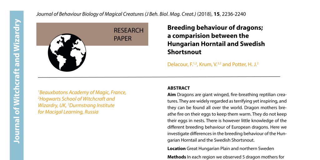
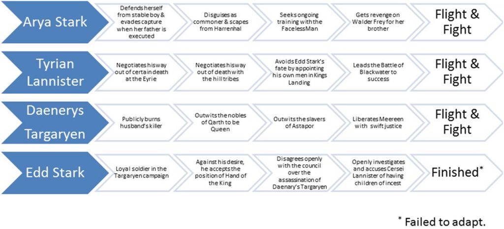
Recently, I came across an article about mortality and survival in Game of Thrones (GoT). The study is published in Injury Epidemiology, examining the survival of 330 main GoT characters, sociodemographic factors, time to death, and circumstances of death. They find that mortality risk is high and characters are more likely to die if they are male and lowborn. The article is a great read including humorous aspects. I started to search for other GoT research and found astonishingly many articles. And there is probably more!
The purpose of the study from Daniel and Westerman (2017) is to determine how people reacted to the end of a parasocial relationship per a character death, by analysing Twitter reactions after the death of fictional character Jon Snow from Game of Thrones. They found that we may respond to a television character’s death in some similar ways as a real person’s. Jules and Lippoff (2016) investigate the dermatological deaseas called Greyscale and compare it to the Hansen disease, or leprosy. And finally, Clapton and Shepherd (2017) show that cultural texts such as GoT can show us different ways of thinking about the world.
There must be more articles that in a serious (or not so much) way try to gain knowledge from a television serious or how we react or interact with/to it. I would love to study some ecological aspect of Game of Thrones. Maybe something about the dragons…
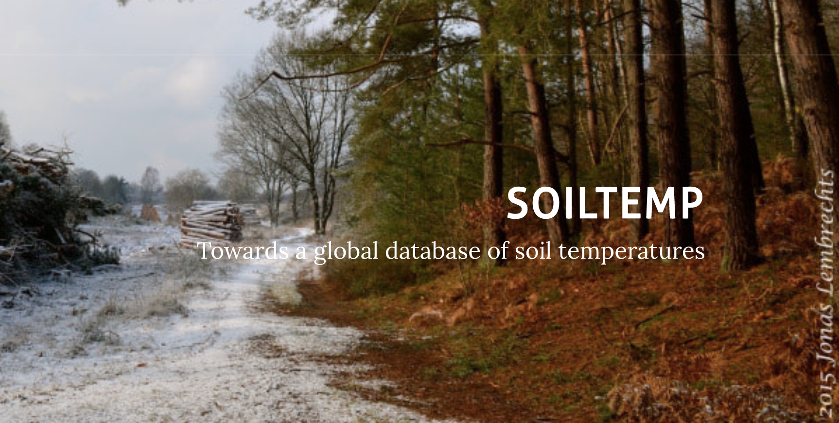
SoilTemp is a new project initiated by Jonas Lambrechts and collegues to create a global soil temperature database. The goal is to make soil temperature data available to scientist, increase and facilitate collaborations across projects and synthesise microclimate data on a global scale to answer key ecological questions.
SoilTemp has recently launched a webpage, where information regarding the data, project updates and future publications can be found. So far they have collected For 1867 temperature sensors from 11 countries, from sea level till 6194 meter above the ocean, and covering more than a decade. And the collection is ongoing.
SeedClim has already provided their long-term (10 years) of soil temperature data. TransPlant, our Chinese Collaborators will follow.